Conditional formatting based on another cell [Google Sheets]

by Matthew Adams

Windows & Software Expert

---

• Google Sheets includes a nifty conditional formatting tool with which you can apply formatting to cells based on specific spreadsheet conditions.
• This guide tells you how users can apply conditional formatting based on another cell in Google Sheets.
• The Teamwork hub includes shortcuts to many other Google app guides.
• Explore our Google Sheets webpage for other useful info on this topic.

Google Sheets includes various formatting options for users. Its users can apply alternative cell color, bold, italic, underline, and font formatting to spreadsheet cells within Sheets.

Those formatting options visually enhance spreadsheets.

Google Sheets also includes a handy conditional formatting tool that enables users to apply selected formatting styles to cells that match a specified condition.

With that tool, you can apply conditional formatting to a selected cell range that’s based on another cell’s value.

How can I use conditional formatting based on another cell in Google Sheets?

1. Apply conditional formatting based on a single cell value

1. First, open a blank spreadsheet in Google Sheets.
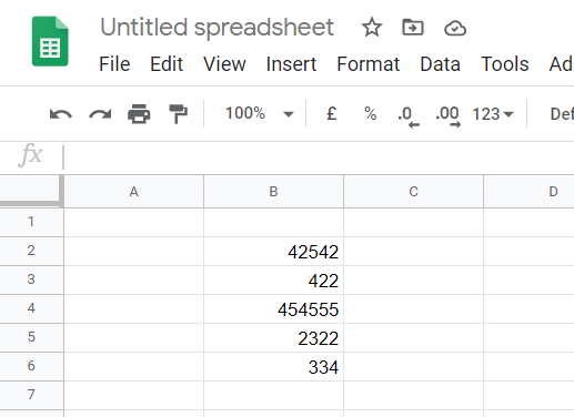
2. Next, enter the dummy data shown in the snapshot directly below within the cell range B2:B5.
   
3. Enter the value 450 within cell C2.
4. Select the cell range B2:B6 by holding the left mouse button and dragging the cursor over them.
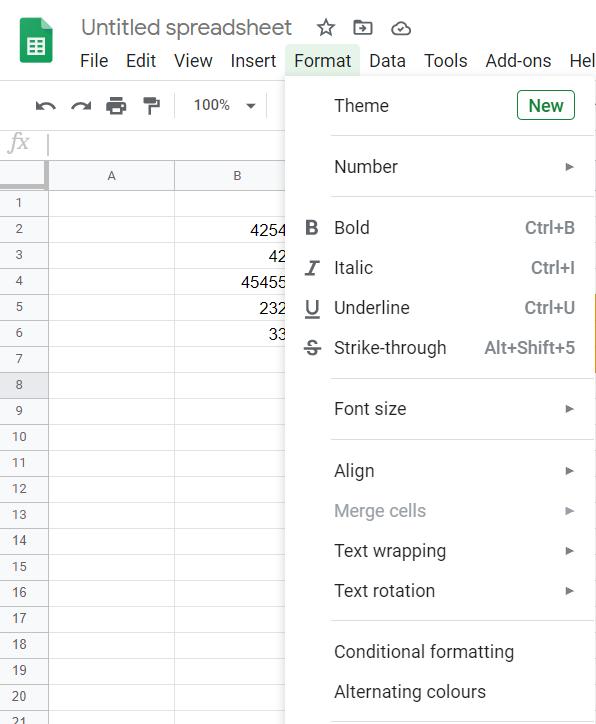
5. Click Format to open that menu.
   
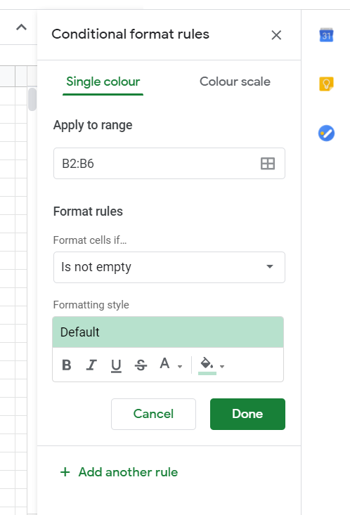
6. Then select Conditional formatting to open the sidebar shown directly below.
   
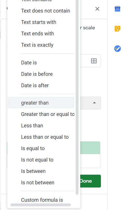
7. Select the greater than option on the Format cells if drop-down menu.
   
8. Enter =C$2 in the Value or formatting text box, which is a reference to cell C2.
9. Click the Fill color button within the Formatting styles box.
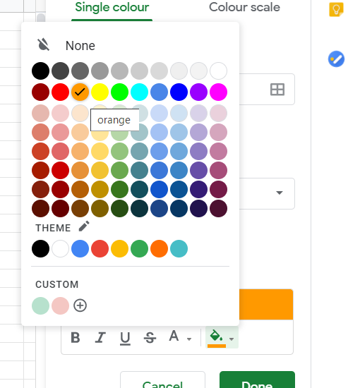
10. Then select the orange color on the palette.
    
11. Click the B Bold button.
12. Press the Done button.

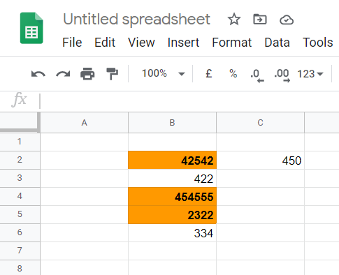
Now cells B2, B4, and B5 within the B2:B6 range will have orange cells and bold text as shown in the screenshot directly below.

Those cells have the selected formatting applied to them as they include higher numbers than the value in C2 the condition is based on.

Note that cell references must always be entered as a formula with = preceding the reference. They must also always include a $ sign between the column letters and row numbers.

You can apply conditional formatting to cells that include dates. For example, you could select the Date is before option to apply formatting to a cell range that includes dates based on a date in a referenced cell.

The Format cells if menu also includes several text options. The Text is exactly option would apply formatting to cells with text that exactly matches that of a referenced one.

---

2. Apply conditional formatting based on multiple cell values across columns

1. Open an empty spreadsheet.
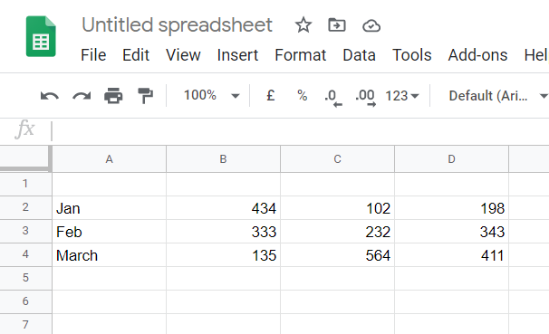
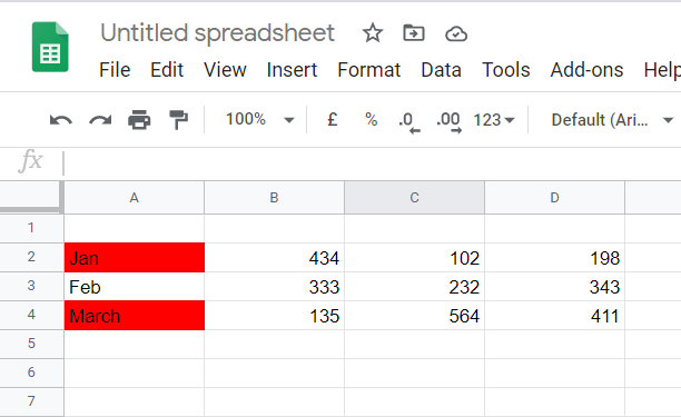
2. Next, enter the dummy data in columns A, B, C, and D exactly as shown in the snapshot directly below.
   
3. Select the cell range A2:A4.
4. Click the Format menu.
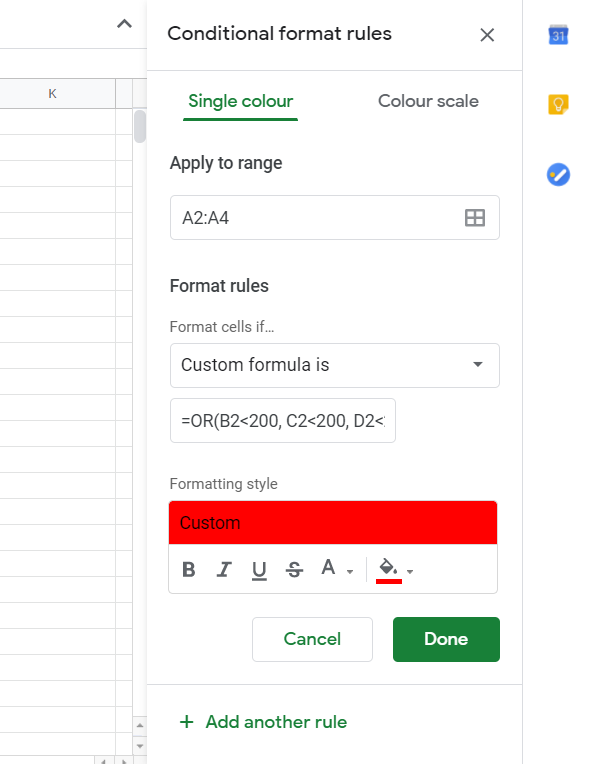
5. Select Conditional formatting to open that tool.
6. Click the Format cells if menu to select Custom formula is.
7. Enter this formula in the Value box: =OR(B2<200, C2<200, D2<200).
   
8. Then click Fill color to select red cell formatting.
9. Click the Done option.

What you’ve done in the example above is to apply red cell formatting to cells A2 and A4 based on all the cell values in their rows (across columns B to D).

As the rows for January and March include cells with values less than 200, red formatting is applied to the Jan and March row headings.

The above examples show you how to apply relatively basic conditional formatting to spreadsheets in Google Sheets.

You can enhance your spreadsheets’ presentation in many ways by applying conditional formatting with custom formulas and the other options on the Format cells if drop-down menu.

Thank you for viewing the article, if you find it interesting, you can support us by buying at the link:: https://officerambo.com/shop/